Usage

Plasticity Phase

import sorn
from sorn import Simulator
import numpy as np

# Sample input
num_features = 10
time_steps = 200
inputs = np.random.rand(num_features,time_steps)

# Simulate the network with default hyperparameters under gaussian white noise
state_dict, E, I, R, C = Simulator.simulate_sorn(inputs = inputs, phase='plasticity',
                                                matrices=None, noise = True,
                                                time_steps=time_steps)

Network Initialized
Number of connections in Wee 3909 , Wei 1574, Wie 8000
Shapes Wee (200, 200) Wei (40, 200) Wie (200, 40)

The default values of the network hyperparameters are,

Hyperparameters of the network and default values

Keyword argument	Value	Description
ne	200	Number of Encitatory neurons in the reservoir
nu	10	Number of Input neurons in the reservoir
network_type_ee	“Sparse”	Sparse or Dense connectivity between Excitatory neurons
network_type_ie	“Dense”	Sparse or Dense connectivity from Excitatory to Inhibitory neurons
network_type_ei	“Sparse”	Sparse or Dense connectivity from Inhibitory to Excitatory neurons
lambda_ee	20	% of connections between neurons in Excitatory pool
lambda_ei	40	% of connections from Inhibitory to Excitatory neurons
lambda_ie	100	% of connections from Excitatory to Inhibitory neurons
eta_stdp	0.004	Hebbian Learning rate for connections between excitatory neurons
eta_inhib	0.001	Hebbian Learning rate for connections from Inhibitory to Excitatory neurons
eta_ip	0.01	Intrinsic plasticity learning rate
te_max	1.0	Maximum excitatory neuron threshold value
ti_max	0.5	Maximum inhibitory neuron threshold value
ti_min	0.0	Minimum inhibitory neuron threshold value
te_min	0.0	Minimum excitatory neuron threshold value
mu_ip	0.01	Target mean firing rate of excitatory neuron
sigma_ip	0.0	Standard deviation of firing rate of excitatory neuron

Override the default hyperparameters and simulate new SORN model

# Sample input
num_features = 5
time_steps = 1000
inputs = np.random.rand(num_features,time_steps)

state_dict, E, I, R, C = Simulator.simulate_sorn(inputs = inputs, phase='plasticity',
                                                matrices=None, noise = True,
                                                time_steps=time_steps,
                                                ne = 100, nu=num_features,
                                                lambda_ee = 10, eta_stdp=0.001)

Network Initialized
Number of connections in Wee 959 , Wei 797, Wie 2000
Shapes Wee (100, 100) Wei (20, 100) Wie (100, 20)

Training phase

from sorn import Trainer
# NOTE: During training phase, input to `sorn` should have second (time) dimension set to 1. ie., input shape should be (input_features,1).

inputs = np.random.rand(num_features,1)

# SORN network is frozen during training phase
state_dict, E, I, R, C = Trainer.train_sorn(inputs = inputs, phase='training',
                                            matrices=state_dict, noise= False,
                                            time_steps=1,
                                            ne = 100, nu=num_features,
                                            lambda_ee = 10, eta_stdp=0.001 )

Freeze plasticity

To turn off any plasticity mechanisms during simulation or training phase, use freeze argument. For example to stop intrinsic plasticity during simulation phase,

# Sample input
num_features = 10
time_steps = 20
inputs = np.random.rand(num_features,time_steps)

state_dict, E, I, R, C = Simulator.simulate_sorn(inputs = inputs, phase='plasticity',
                                                matrices=None, noise = True,
                                                time_steps=time_steps, ne = 50,
                                                nu=num_features, freeze=['ip'])

To train the above model under plasticity mechanisms except ip and istdp, use freeze argument

state_dict, E, I, R, C = Trainer.train_sorn(inputs = inputs, phase='plasticity',
                                            matrices=state_dict, noise= False,
                                            time_steps=1,
                                            ne = 50, nu=num_features,
                                            freeze=['ip','istdp'])

To train the above model with all plasticity mechanisms frozen , change the phase argument value to training

state_dict, E, I, R, C = Trainer.train_sorn(inputs = inputs, phase='training',
                                            matrices=state_dict, noise= False,
                                            time_steps=1,
                                            ne = 50, nu=num_features)

The other options are,

stdp - Spike Timing Dependent Plasticity

ss - Synaptic Scaling

sp - Structural Plasticity

istdp - Inhibitory Spike Timing Dependent Plasticity

Note: If you pass all above options to freeze, then the network will behave as Liquid State Machine(LSM) i,e., the connection strengths and thresholds remains fixed at the random intial state.

Network Output Descriptions

state_dict - Dictionary of connection weights (Wee,`Wei`,`Wie`) ,

Excitatory network activity (X),

Inhibitory network activities(Y),

Threshold values (Te,`Ti`)

E - Excitatory network activity of entire simulation period

I - Inhibitory network activity of entire simulation period

R - Recurrent network activity of entire simulation period

C - Number of active connections in the Excitatory pool at each time step

Colaboratory Notebook

Sample simulation and training runs with few plotting functions are found at Colab

Usage with OpenAI gym

Cartpole balance problem

from sorn import Simulator, Trainer
import gym

# Hyperparameters
NUM_EPISODES = int(2e6)
NUM_PLASTICITY_EPISODES = 20

LEARNING_RATE = 0.0001 # Gradient ascent learning rate
GAMMA = 0.99 # Discounting factor for the Rewards

# Open AI gym; Cartpole Environment
env = gym.make('CartPole-v0')
action_space = env.action_space.n

# SORN network parameters
ne = 50
nu = 4
# Init SORN using Simulator under random input;
state_dict, E, I, R, C = Simulator.simulate_sorn(inputs = np.random.randn(4,1),
                                                phase ='plasticity',
                                                time_steps = 1,
                                                noise=False,
                                                ne = ne, nu=nu)

w = np.random.rand(ne, 2) # Output layer weights

# Policy
def policy(state,w):
    "Implementation of softmax policy"
    z = state.dot(w)
    exp = np.exp(z)
    return exp/np.sum(exp)

# Vectorized softmax Jacobian
def softmax_grad(softmax):
    s = softmax.reshape(-1,1)
    return np.diagflat(s) - np.dot(s, s.T)

for EPISODE in range(NUM_EPISODES):

    # Environment observation;
    # NOTE: Input to sorn should have time dimension. ie., input shape should be (input_features,time_steps)
    state = env.reset()[:, None] # (4,) --> (4,1)

    grads = [] # Episode log policy gradients
    rewards = [] # Episode rewards

    # Keep track of total score
    score = 0

    # Play the episode
    while True:

      # env.render() # Uncomment to see your model train in real time (slow down training progress)
      if EPISODE < NUM_PLASTICITY_EPISODES:

        # Plasticity phase
        state_dict, E, I, R, C = Simulator.simulate_sorn(inputs = state, phase ='plasticity',
                                                        matrices = state_dict, time_steps = 1,
                                                        ne = ne, nu=nu,
                                                        noise=False)

      else:
        # Training phase with frozen reservoir connectivity
        state_dict, E, I, R, C = Trainer.train_sorn(inputs = state, phase = 'training',
                                                matrices = state_dict, time_steps = 1,
                                                ne = ne, nu=nu,
                                                noise= False)

      # Feed E as input states to your RL algorithm, below goes for simple policy gradient algorithm
      # Sample policy w.r.t excitatory states and take action in the environment
      probs = policy(np.asarray(E),w)
      action = np.random.choice(action_space,p=probs[0])
      state,reward,done,_ = env.step(action)
      state = state[:,None]

      # COMPUTE GRADIENTS BASED ON YOUR OBJECTIVE FUNCTION;
      # Sample computation of policy gradient objective function
      dsoftmax = softmax_grad(probs)[action,:]
      dlog = dsoftmax / probs[0,action]
      grad = np.asarray(E).T.dot(dlog[None,:])
      grads.append(grad)
      rewards.append(reward)
      score+=reward

      if done:
          break

    # OPTIMIZE OUTPUT LAYER WEIGHTS `w` BASED ON YOUR OPTIMIZATION METHOD;
    # Below is a sample of weight update based on gradient ascent(maximize cumulative reward) method for temporal difference learning
    for i in range(len(grads)):

        # Loop through everything that happened in the episode and update towards the log policy gradient times future reward
        w += LEARNING_RATE * grads[i] * sum([ r * (GAMMA ** r) for t,r in enumerate(rewards[i:])])
    print('Episode %s  Score %s' %(str(EPISODE),str(score)))

There are several neural data analysis and visualization methods inbuilt with sorn package. Sample call for few plotting and statistical methods are shown below;

Plotting functions

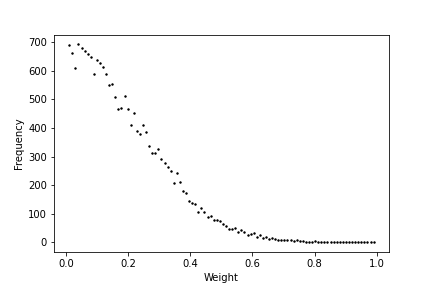
Plot weight distribution in the network

from sorn import Plotter
# For example, the network has 200 neurons in the excitatory pool.
Wee = np.random.randn(200,200) # Note that generally Wee is sparse
Wee=Wee/Wee.max() # state_dict['Wee'] returned by the SORN is already normalized
Plotter.weight_distribution(weights= Wee, bin_size = 5, savefig = True)

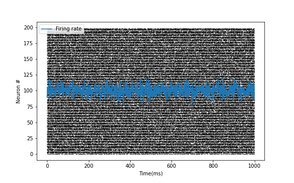
Plot Spike train

E = np.random.randint(2, size=(200,1000)) # For example, activity of 200 excitatory neurons in 1000 time steps
Plotter.scatter_plot(spike_train = E, savefig=True)

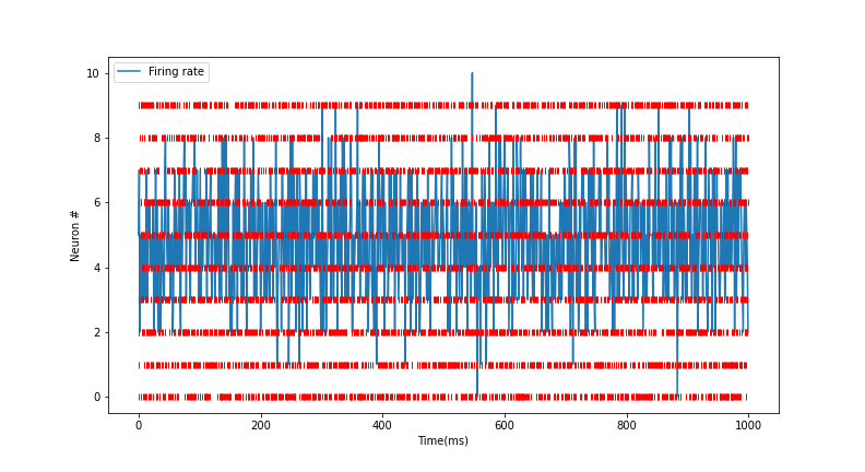
Raster plot of Spike train

# Raster plot of activity of only first 10 neurons in the excitatory pool
Plotter.raster_plot(spike_train = E[:,0:10], savefig=True)

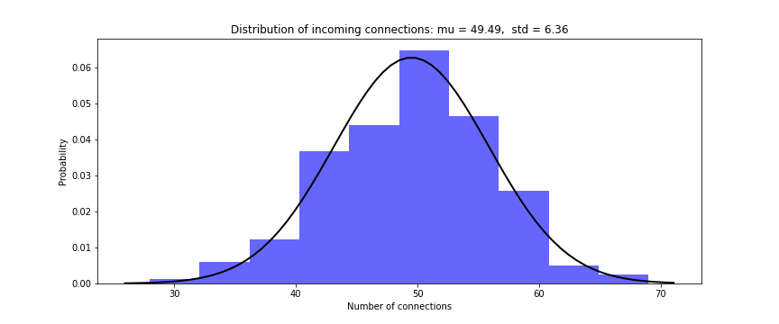
Distribution of presynaptic connections

# Histogram of number of presynaptic connections per neuron in the excitatory pool
Plotter.hist_incoming_conn(weights=Wee, bin_size=10, histtype='bar', savefig=True)

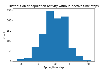
Distribution of firing rate of the network

Plotter.hist_firing_rate_network(E, bin_size=10, savefig=True)

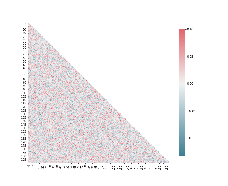
Plot pearson correlation between neurons

from sorn import Statistics
avg_corr_coeff,_ = Statistics.avg_corr_coeff(E)
Plotter.correlation(avg_corr_coeff,savefig=True)

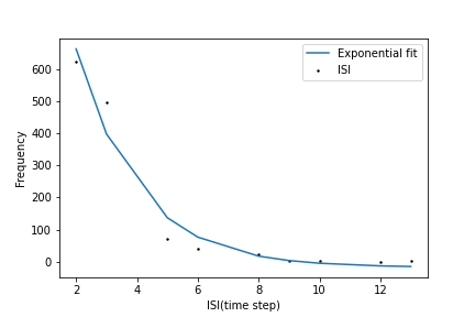
Inter spike intervals

# Inter spike intervals with exponential curve fit for neuron 1 in the Excitatory pool
Plotter.isi_exponential_fit(E,neuron=1,bin_size=10, savefig=True)

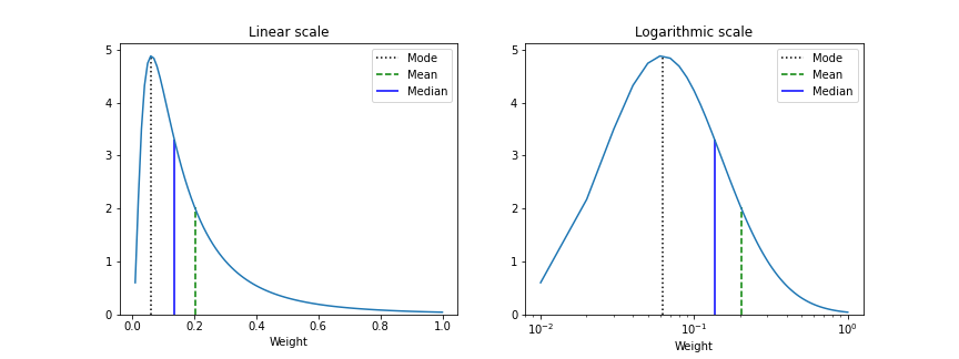
Linear and Lognormal curve fit of Synaptic weights

# Distribution of connection weights in linear and lognormal scale
Plotter.linear_lognormal_fit(weights=Wee,num_points=100, savefig=True)

Network plot

# Draw network connectivity using the pearson correlation function between neurons in the excitatory pool
Plotter.plot_network(avg_corr_coeff,corr_thres=0.01,fig_name='network.png')

Statistics and Analysis functions

t-lagged auto correlation between neural activity

from sorn import Statistics
pearson_corr_matrix = Statistics.autocorr(firing_rates = [1,1,5,6,3,7], t= 2)

Fano factor

# To verify poissonian process in spike generation of neuron 10
mean_firing_rate, variance_firing_rate, fano_factor = Statistics.fanofactor(spike_train= E,
                                                                        neuron = 10,
                                                                        window_size = 10)

Spike Source Entropy

# Measure the uncertainty about the origin of spike from the network using entropy
sse = Statistics.spike_source_entropy(spike_train= E, num_neurons=200)